Assignment: Xarray Fundamentals with Atmospheric Radiation Data

Assignment: Xarray Fundamentals with Atmospheric Radiation Data#

In this assignment, we will use Xarray to analyze top-of-atmosphere radiation data from NASA’s CERES project.

Public domain, by NASA, from Wikimedia Commons

A pre-downloaded and subsetted a portion of the CERES dataset is available here: http://ldeo.columbia.edu/~danielmw/CERES_EBAF-TOA_Edition4.0_200003-201701.condensed.nc. The size of the data file is 702.53 MB. It may take a few minutes to download.

Please review the CERES FAQs before getting started.

Start by importing Numpy, Matplotlib, and Xarray. Set the default figure size to (12, 6).

import xarray as xr
import numpy as np
from matplotlib import pyplot as plt
plt.rcParams['figure.figsize'] = (12, 6)

Next, download the NetCDF file using pooch.

import pooch
fname = pooch.retrieve(
    'http://ldeo.columbia.edu/~danielmw/CERES_EBAF-TOA_Edition4.0_200003-201701.condensed.nc',
    known_hash=None,  downloader=pooch.HTTPDownloader(verify=False)
)
print(fname)

Downloading data from 'http://ldeo.columbia.edu/~danielmw/CERES_EBAF-TOA_Edition4.0_200003-201701.condensed.nc' to file '/Users/danielmw/Library/Caches/pooch/a379a4cf37bf10809e636b0809c1c88b-CERES_EBAF-TOA_Edition4.0_200003-201701.condensed.nc'.
/opt/anaconda3/lib/python3.13/site-packages/urllib3/connectionpool.py:1097: InsecureRequestWarning: Unverified HTTPS request is being made to host 'ldeo.columbia.edu'. Adding certificate verification is strongly advised. See: https://urllib3.readthedocs.io/en/latest/advanced-usage.html#tls-warnings
  warnings.warn(
/opt/anaconda3/lib/python3.13/site-packages/urllib3/connectionpool.py:1097: InsecureRequestWarning: Unverified HTTPS request is being made to host 'www.ldeo.columbia.edu'. Adding certificate verification is strongly advised. See: https://urllib3.readthedocs.io/en/latest/advanced-usage.html#tls-warnings
  warnings.warn(
SHA256 hash of downloaded file: a876cc7106e7dcb1344fbec5dcd7510e5cd947e62049a8cbc188ad05ffe00345
Use this value as the 'known_hash' argument of 'pooch.retrieve' to ensure that the file hasn't changed if it is downloaded again in the future.

/Users/danielmw/Library/Caches/pooch/a379a4cf37bf10809e636b0809c1c88b-CERES_EBAF-TOA_Edition4.0_200003-201701.condensed.nc

1) Opening data and examining metadata#

1.1) Open the dataset and display its contents#

1.2) Print out the `long_name` attribute of each variable#

Print variable: long name for each variable. Format the output so that the start of the long name attributes are aligned.

2) Basic reductions, arithmetic, and plotting#

2.1) Calculate the time-mean of the entire dataset#

2.2) From this, make a 2D plot of the the time-mean Top of Atmosphere (TOA) Longwave, Shortwave, and Incoming Solar Radiation#

(Use “All-Sky” conditions)

Note the sign conventions on each variable.

2.3) Add up the three variables above and verify (visually) that they are equivalent to the TOA net flux#

You have to pay attention to and think carefully about the sign conventions (positive or negative) for each variable in order for the variables to sum to the right TOA net flux. Refer to the NASA figure at the top of the page to understand incoming and outgoing radiation.

3) Mean and weighted mean#

3.1) Calculate the global (unweighted) mean of TOA net radiation#

Since the Earth is approximately in radiative balance, the net TOA radiation should be zero. But taking the naive mean from this dataset, you should find a number far from zero. Why?

The answer is that each “pixel” or “grid point” of this dataset does not represent an equal area of Earth’s surface. So naively taking the mean, i.e. giving equal weight to each point, gives the wrong answer.

On a lat / lon grid, the relative area of each grid point is proportional to \(\cos(\lambda)\). (\(\lambda\) is latitude)

3.2) Create a `weight` array proportional to \(\cos(\lambda)\)#

Think carefully a about radians vs. degrees

3.3) Redo your global mean TOA net radiation calculation with this weight factor#

Use xarray’s weighted array reductions to compute the weighted mean.

This time around, you should have found something much closer to zero. Ask a climate scientist what the net energy imbalance of Earth due to global warming is estimated to be. Do you think our calculation is precise enough to detect this?

3.4) Now that you have a `weight` factor, verify that the TOA incoming solar, outgoing longwave, and outgoing shortwave approximately match up with infographic shown in the first cell of this assignment#

4) Meridional Heat Transport Calculation#

We can go beyond a weight factor and actually calculate the area of each pixel of the dataset, using the formula

\[ dA = R^2 \cos(\lambda) d\lambda d \varphi \]

where \(d\lambda\) and \(d\varphi\) are the spacing of the points in latitude and longitude (measured in radians). We can approximate Earth’s radius as \(R = 6,371\) km.

4.1) calculate the pixel area using this formula and create a 2D (lon, lat) DataArray for it#

(Xarray’s ones_like function can help you easily create and broadcast DataArrays.) Verify that the sum of all the pixels equals the Earth’s true surface area as evaluated using the formula for the area of a sphere (yes, the Earth is not a sphere … it’s just a homework problem).

4.2) Calculate and plot the total amount of net radiation in each 1-degree latitude band#

Multiplying the pixel area (m\(^2\)) from above with the radiative flux (W m\(^{-2}\)) gives you the total amount of radiation absorbed in each pixel in W.

Label with correct units.

4.3) Plot the cumulative sum of the total amount of net radiation as a function of latitude#

Label with correct units. (Hint: check out xarray’s cumsum function.)

This curve tells you how much energy must be transported meridionally by the ocean and atmosphere in order to account for the radiative imbalance at the top of the atmosphere.

You should get a curve that looks something like this: https://journals.ametsoc.org/view/journals/clim/14/16/full-i1520-0442-14-16-3433-f07.gif (Figure from Trenberth & Caron, 2001)

5) Making Maps with Cartopy#

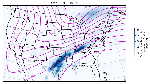
5.1) Plot data from NARR#

NARR is NCEP’s North American Regional Reanalysis, a widely used product for studying the weather and climate of the continental US. The data is available from NOAA’s Earth System Research Laboratory via OPeNDAP, meaing that xarray can open the data “remotely” without downloading a file.

For this problem, you should open this geopential height file:

https://www.esrl.noaa.gov/psd/thredds/dodsC/Datasets/NARR/Dailies/pressure/hgt.201810.nc

And this precipitation file:

https://www.esrl.noaa.gov/psd/thredds/dodsC/Datasets/NARR/Dailies/monolevel/apcp.2018.nc

Your goal is to make a map that looks like the one below. It shows total precipitation on Oct. 15, 2018 in blue, plus contours of the 500 mb geopotential surface.

Hint: examine the dataset variables and attirbutes carefully in order to determine the projection of the data.

narr_map

url = "https://www.esrl.noaa.gov/psd/thredds/dodsC/Datasets/NARR/Dailies/pressure/hgt.201810.nc"
ds = xr.open_dataset(url, engine="netcdf4")

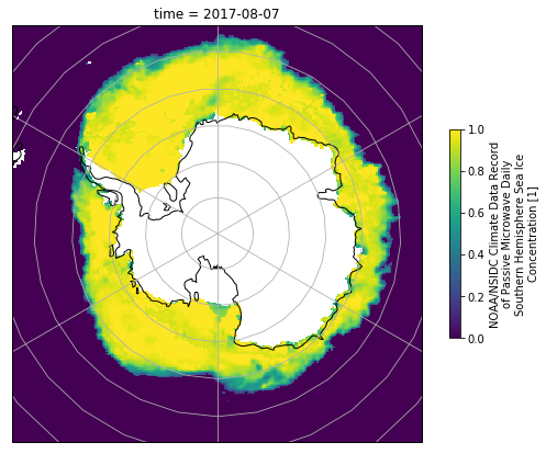
5.2) Antarctic Sea Ice#

Download this file and then use it to plot the concentration of Antarctic Sea Ice on Aug. 7, 2017. Again, you will need to explore the file contents in order to determine the correct projection.

import xarray as xr
import pooch
url = 'https://polarwatch.noaa.gov/erddap/files/nsidcCDRiceSQsh1day/2017/seaice_conc_daily_sh_f17_20170807_v03r01.nc'
fname = pooch.retrieve(url, known_hash='19b74e7e97f1c0786da0c674c4d5e4af0da5b32e2fe8c66a8f1a8a9a1241e73c')
ds_ice = xr.open_dataset(fname, drop_variables='melt_onset_day_seaice_conc_cdr')

sea_ice_map

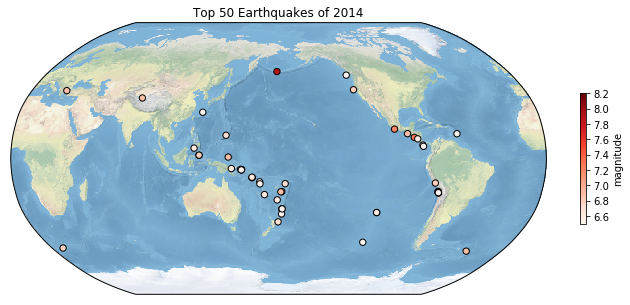
5.3) Global USGS Earthquakes#

Reload the file we explored in homework 5 using pandas

http://www.ldeo.columbia.edu/~danielmw/usgs_earthquakes_2014.csv

and use the data to recreate this map.

earthquake_map